

Multitrait GWAS: Why can combining traits improve power?
10th August 2024
Why combine traits?
When you are interested in the genetic basis of traits that are correlated with one another it can often be helpful to analyse those traits together in some kind of multitrait genome-wide-association (GWA) study.
However, the reasons for why a multivariate analysis might increase statistical power are not very intuitive, and it can be hard to find answers online about why a joint analysis may be useful. Here I want to illustrate why this works. This will not be formally correct, rather I want to build an intuition for what a multivariate analysis is and how it affects the statistics.
It’s also important to be aware that a joint analysis may not help. I strongly recommend reading the introduction and the first section of the methods in Matthew Stephens’ excellent paper on when a multitrait does or does not improve statistical power.
Univariate and multivariate tests
In a standard GWAS, we test the association between a single phenotype (let’s call it trait X), and each SNP in turn. This is like any classical statistical test - you estimate an observed statistical test, and compare it to the expected null distribution (see A in the figure below). The p-value is the area under the curve of the null distribution beyond the value of the test statistic. This is called a univariate test, because there is only one association to test, and we can plot the observed and null distributions along a single axis. Let’s imagine that the p-value from this analysis was 0.1 - close, but not quite significant.
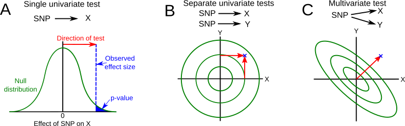
If we have two traits (called them traits X and Y), we could just run two separate univariate analyses (subfigure B). The red lines show the effects of an allele that increases both X and Y, and is shown in two dimensions. The null distribution is also in two dimensions, so this is shown as contour lines of increasing density, with the highest density at the centre. There are two separate tests, asking whether the effect sizes (red arrows) are different from zero. If we imagine that the outermost contour is the 95% quantile of that two-dimensional distribution, we can see that neither effect size is significant.
However, treating X and Y as independent ignores information about the correlation between them. Specifically, we ignore the correlation between errors. This refers to the variation which is not due to the effects of the SNP we are looking at, which you may also have heard referred to a ‘residuals’ or ‘residual errors’. This correlation matters because it affects the shape of the null distribution (subfigure C). In this case, residual errors are negatively correlated, so the null distribution is now longer along one diagonal axis than the other. That means that the bivariate effect size of the association with X and Y now falls outside of the null distribution, and is now significant.
Importantly neither the values for effect sizes, nor the overall width and height of the null distribution have not changed (although I realise this may not be clear from how I’ve drawn it). All that has changed is the shape of the null distribution, and therefore the p-values.